Introduction
Despite numerous regulatory efforts for greater transparency, the nature of the municipal bond market remains opaque due to its fragmented nature. While some of the attempts at increasing transparency such as municipal issuer continuing disclosure requirements or near-real time trade data reporting have been effective, even with 30,000+ trades reported daily, publicly available trade data fails to provide meaningful context for price discovery of municipal securities without extensive manipulation. And even though they may appear to be alike, no two municipal bonds are directly comparable due to the innate diversity of municipal issuers. For many investment professionals, it is difficult to establish the relative value of securities in which they wish to invest. The problem is magnified for the end investor.
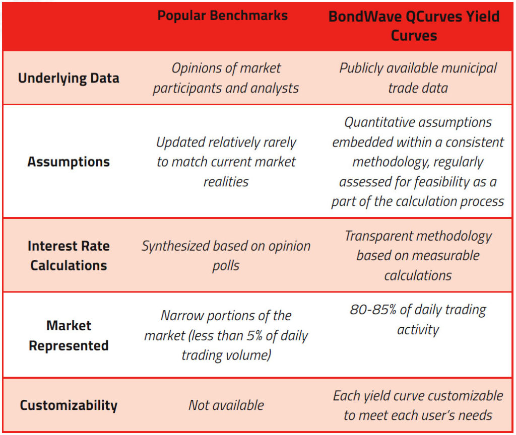
Existing solutions fall into two broad categories: benchmarks (i.e. yield curves) and indices. Between the two they provide some framework, but do not necessarily equip the investors with a transparent or complete engine to ease their search for value. For example, popular municipal yield curves use polling techniques to establish an opinion of value (rather than observable market data) and do so over a very small slice of the municipal market. One such curve is limited to bonds rated AAA with a 5% coupon, which represent less than 2% of daily trading in municipal bonds. Another uses a single state (Maryland) and bond characteristic (general obligation) as a general guide. While these simplifications are appealing in that they remove complications from the calculations, they do not make for a more comprehensive depiction of the actual market. With today’s large, detailed databases, improved hardware and software techniques for dealing with masses of data, it is time to revisit the need for simplifications that remove available data from calculations.
Indices represent a greater portion of the municipal market and are designed to be broadly inclusive. This inclusive nature means that they will include securities which are not available for purchase. As such, they wholly depend on third party evaluations. And unlike yield curves, indices are primarily used as benchmarks for portfolio total returns rather than facilitating daily trading or investment related decisions by allowing comparisons across bonds at a point in time.
In either case, with current yield curves or indices there is an inherent bias and lack of transparency because neither of the benchmarks are based on actual market observations. What then does the market need?
Emerging technology tools can enable traders and investors to address this problem through a transparent, quantitative and flexible approach utilizing newly publicly available trade data. These state-of-the-art solutions include the fixed coupon investment grade segment of the tax exempt municipal market (representing 80-85% of daily municipal trading activity), and provides what BondWave believes is just the right amount of context to municipal price discovery.
Municipal Benchmarks
In the contemporary municipal market, predominantly two types of benchmarks influence the determination of general level of interest rates:
- Yield Curves – the term structure of interest rates, representing the relation between yield levels and maturities at a point in time; and
- Bond Indices – a broad rules-based composite used to determine value of a certain bond market segment over time, regardless of the underlying constituent maturities.
While they influence trading patterns, investment decisions and relative value, most popular yield curves and indices have a few common weaknesses which an investor alone cannot overcome.
Prevailing yield curves are defined by a specific set of criteria – such as coupon rate, rating or sector. These criteria, as in the earlier examples, usually define a very narrow portion of the market. The underlying assumptions are also very rarely updated to reflect current trading behavior. The calculated yields are synthesized and updated based on opinions of analysts and market participants introducing the potential for bias into the calculations. The potential for bias can be removed by a properly constructed yield curve that relies on the truest expression of value: arm’s length transactions between informed market participants. Historically, this proved impossible prior to the advent of the near real-time reporting of all trades to a publicly available database. More recently it proved inconvenient because the organization, size and diversity of that database made analysis difficult. However, with improved tools for analysis, consumption, and organization of near real-time trade data it is time to update yield curve techniques to reflect these realities.
Bond indices are slightly different. They are more inclusive in nature and provide ways to group similar securities via a set of inclusion and exclusion rules. A few popular indices consider the entire bond universe when creating such groups, while others focus on a much smaller set of issuers (or specific securities). This subjects them to the ‘narrowness bias’ not unlike the yield curves. When it comes to valuation, indices are not valued based on opinions; but nor are they valued based on actual observable market data. Indices are valued based on theoretical evaluated prices of their constituent securities or estimates from market participants. Therefore, performance of the indices is influenced by the inclusion of a few large issuers regardless of whether those large issues trade in the market.
On-the-run or bellwether securities could also be potential benchmark options, but it is not a notion that fits in the municipal market. Unlike the US Treasury market, defining such a benchmark for municipal securities is a difficult task because of the diverse nature of issuers and the wealth of possible structures. Not all municipal issuers have sufficient debt outstanding to provide the necessary liquidity. And while there is no lack of trade volume on any given day, it is difficult to find a single security which trades consistently enough to be defined as a benchmark. Regulatory (bank qualified securities, disclosure rules, etc.) and other market forces (state/municipal budget deadlines, availability of funding, early redemptions, etc.) heavily influence which bonds are available for purchase. That makes it nearly impossible to come up with something akin to a set of ‘on-the-run’ or bellwether securities as benchmark.
How does one get beyond the shortcomings of existing benchmarks to arrive at meaningful conclusions?
Why Guess When We Can Measure?
We have at our disposal accurate, comprehensive, publicly available trade data published by MSRB. It holds immense potential to be analyzed numerous ways to create observable quantitative benchmarks. Such an approach can make up for the inadequacies of prevailing benchmarks by being:
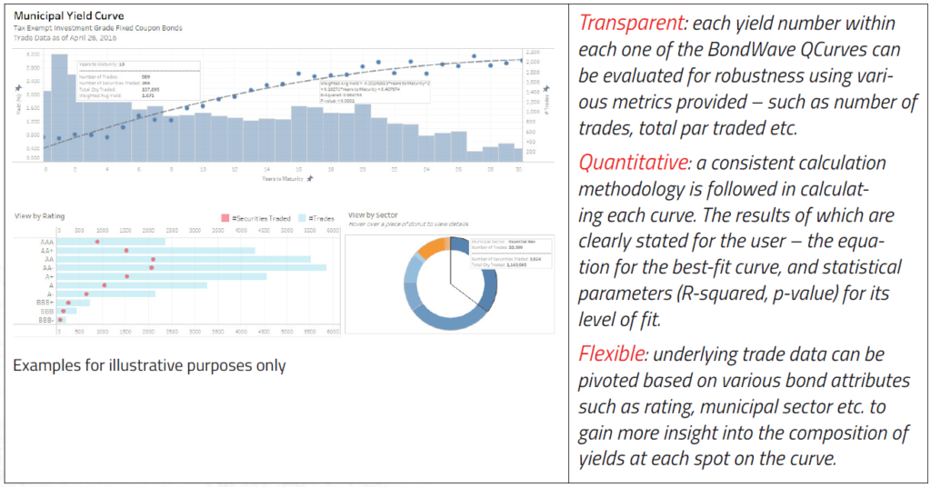
- transparent (based on an observable dataset),
- quantitative (methodology based on measurable calculations as opposed to opinions), and
- flexible (enough to provide investors with ways to navigate the murky waters of municipal relative value analysis).
At BondWave Labs, we’ve developed solutions to create yield curves that meet all three of these criteria.
The first step was creating a consistent quantitative methodology based on publicly available municipal trade data to deliver yield context. Various clusters of trades are formed, where each cluster has its own unique set of ‘similarity’ characteristics. Each of these clusters can be thought of as a distinct ‘Bond Type’.
Trades within each given Bond Type can be meaningfully compared to one another. A user can also map any given security to one of these Bond Types based on relevant set of characteristics. Additionally, with these newly available tools, users can create customized versions of the available yield curves tailored to their needs – introducing immense flexibility in the analysis they wish to carry out.
BondWave QCurves Yield Curves: Design and Methodology
The methodology behind BondWave QCurves takes a consistent data-centric, transparent approach to development of yield curves. The basis for yield calculations is publicly available municipal trade data obtained from MSRB. This dataset is examined daily for irregularities and carefully analyzed for inaccuracies.
- Bond descriptive elements such as municipal sector, rating, coupon type and state of issue of the security are used to divide trade data into distinct clusters (or Bond Types).
- Zero coupon bonds are excluded from the analysis. They usually trade at a deep discount, and have a unique duration/return dynamic due to their non-coupon paying nature, thus demonstrating a trading behavior that is fundamentally different from their fixed coupon paying counterparts.
- All three trade types (dealer to dealer, purchase from customer and sale to customer) and all trade sizes are included in preliminary yield calculations. Users have the flexibility to choose between the three trade types and relevant groups of trade sizes to meet their analysis requirements.
- Trades are further grouped by years to maturity within each cluster.
- Minimum data requirements1 are imposed per maturity year to ensure that yield curve calculations are meaningful. Additionally, a quartile-based outlier removal method2 is applied to each maturity subset within each trade cluster so that the resulting interest rates remain neutral to extreme observations.
- Interest rate levels weighted by trade size are calculated from these standardized datasets for the entire term structure, and a ‘best fit’ curve is also derived. For this, we employ a second order polynomial equation to determine a graphical curve that represents the interest rates accurately.
- As an important step taken towards improving transparency in benchmark calculations, the metrics indicative of the depth of data of any given point are displayed. These metrics include, but are not limited to, number of trades, total par traded, number of unique securities traded, R-squared3 value and p-value4 for the best fit curve.
17 unique yield curves are offered at present:
- Tax Exempt Investment Grade Municipal Benchmark
- Sector Specific Yield Curves
a) Essential Revenue Securities
b) Essential Unlimited General Obligation Securities
c) Essential Limited GO and Double Barreled Securities
d) Essential Tax, Lease Revenue and Federal Grant Securities
e) Nonessential Revenue Securities - State Specific Yield Curves
a) California
b) Florida
c) New Jersey
d) New York
e) Pennsylvania
f) Texas - Rating Specific Yield Curves
a) AAA Rated Securities
b) AA Rated Securities
c) A Rated Securities
d) BBB Rated Securities - Other Yield Curves
a) Pre-refunded Securities
BondWave QCurves Yield Curves will help users drive their search for value both for a specific security, and across the spectrum of these curves. Because of the consistent methodology, these benchmarks can be meaningfully compared to one another at any point in time. They can also be used to understand the trends in municipal yields over time.
A transparent data centric methodology, attractive visual display of calculated data, and intuitive quick filters which provide alternative views of the traded securities should empower the user with material insights into price/yield levels of tax exempt municipal securities.
This material has been prepared by BondWave LLC (BondWave) and reflects the current opinion of the authors. It is based on sources and data believed to be accurate and reliable but has not been independently verified by BondWave. Opinions and forward looking statements are subject to change without notice. The material does not constitute a research report or advice and any securities referenced are for illustrative purposes only and not a recommendation to buy or sell any security.
1 A minimum of 30 trades need to be available in more than 10 unique securities to calculate a meaningful yield for a given maturity within a trade cluster.
2 Any yield below Q1-1.5*Q1 or above Q3+1.5*Q3 is considered an outlier, and corresponding trade left out of the analysis.
3 R-squared value (the “coefficient of determination”) is a statistic which indicates the strength of fit of the ‘best fit’ yield curve. In other words, it specifies the percentage of sample data that can be explained by the derived best fit curve. The highest possible R-squared value for any fitted curve is “1”, indicating a perfect fit.
4 p-value (the “level of significance”) indicates the probability that the best fit curve equation will fail to predict an accurate yield for a given point on the term structure for the given data sample. A lower p-value means a best fit curve which is better at describing the underlying yield trends.
